Control Chart, Limits, Types and Formulas - Revision Notes

Control chart

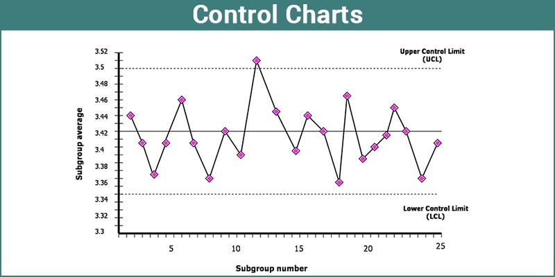
Control charts are graphical tools used in statistical process control to monitor processes over time and detect any unusual variation or patterns. They help in understanding the stability and predictability of a process by displaying data points plotted in time order along with control limits.

Limits in Control Charts

In control charts, limits are established to distinguish between common cause variation (normal variation inherent in the process) and special cause variation (variation due to specific, identifiable reasons). The two main types of limits are:

1. Upper Control Limit (UCL): This is the upper boundary line on a control chart, representing the highest acceptable value for the process. Data points above this limit indicate potential special causes of variation that require investigation and corrective action.
2. Lower Control Limit (LCL): This is the lower boundary line on a control chart, representing the lowest acceptable value for the process. Data points below this limit also suggest potential special causes of variation.

Types of Control Chart

There are different types of control charts, including variable control charts and attribute control charts:

→ Variable Control Charts: These are used when the data collected is in the form of continuous measurements, such as length, weight, or volume. Variable control charts include:
X-Bar (Mean) Chart: Monitors the central tendency or average of a process over time.
R (Range) Chart: Tracks the variability or spread of data within a sample over time.

→ Attribute Control Charts: These are used when data is in the form of counts or categories, such as the number of defects, pass/fail outcomes, etc. Attribute control charts include:
P (Proportion) Chart: Used to monitor the proportion of defective items in a sample.
C (Count) Chart: Tracks the number of defects or occurrences of a specific attribute in a sample.

Formulas for Control Chart Limits

The formulas for calculating control chart limits depend on the type of control chart being used:

1. Variable Control Charts:
→ For X-Bar (Mean) Chart:
$UCL = \bar{X} + A_2 \times \bar{R}$
$LCL = \bar{X} - A_2 \times \bar{R}$

→ For R (Range) Chart:
$UCL = D_4 \times \bar{R}$
$LCL = D_3 \times \bar{R}$

2. Attribute Control Charts:
→ For P (Proportion) Chart:
$UCL = \hat{p} + Z \times \sqrt{\frac{\hat{p}(1-\hat{p})}{n}}$
$LCL = \hat{p} - Z \times \sqrt{\frac{\hat{p}(1-\hat{p})}{n}}$

→ For C (Count) Chart:
$UCL = c + 3\sqrt{c}$
$LCL = c - 3\sqrt{c}$

Here, $\bar{X}$ represents the average of sample means, $\bar{R}$ is the average range within samples, $\hat{p}$ is the average proportion of defects, $n$ is the sample size, and $Z$ is the Z-score corresponding to the desired confidence level. The values of $A_2$, $D_3$, and $D_4$ are constants obtained from statistical tables.

Example Question

A football manufacturing company wants to check the variation in the weight of balls. For this, 25 samples (each of size 4) are selected. The weight of each ball is measured (in grams), the sum of sample averages and sum of sample ranges were found to be $\sum_{i=1}^{25} \bar{x}_i = 4010$ grams and $\sum_{i=1}^{25} R_i = 72$ grams, respectively. Compute the control limits for the $\bar{X}$ and R-chart. It is given that $A2 = 0.729$, $D3 = 0$ and $D4 = 2.282$ .

Answer:

Given:

Number of samples ($k$) = 25
Sample size ($n$) = 4
Sum of sample averages ($\sum_{i=1}^{25} \bar{x}_i$) = 4010 grams
Sum of sample ranges ($\sum_{i=1}^{25} R_i$) = 72 grams
Constants: $A2 = 0.729$, $D3 = 0$, $D4 = 2.282$

Step-by-Step Solution:

1. Calculate the average of sample means ($\bar{\bar{x}}$):
$\bar{\bar{x}} = \frac{\sum_{i=1}^{25} \bar{x}_i}{25} = \frac{4010}{25} = 160.4 \text{ grams}$

2. Calculate the average range ($\bar{R}$):
$\bar{R} = \frac{\sum_{i=1}^{25} R_i}{25} = \frac{72}{25} = 2.88 \text{ grams}$

3. Control Limits for $\bar{X}$-Chart:
The control limits for the $\bar{X}$-chart are calculated as follows:

Upper Control Limit (UCL):
$\text{UCL}_{\bar{X}} = \bar{\bar{x}} + A2 \cdot \bar{R}$
$\text{UCL}_{\bar{X}} = 160.4 + 0.729 \cdot 2.88 = 160.4 + 2.10032 = 162.50032 \text{ grams}$

Center Line (CL):
$\text{CL}_{\bar{X}} = \bar{\bar{x}} = 160.4 \text{ grams}$

Lower Control Limit (LCL):
$\text{LCL}_{\bar{X}} = \bar{\bar{x}} - A2 \cdot \bar{R}$
$\text{LCL}_{\bar{X}} = 160.4 - 0.729 \cdot 2.88 = 160.4 - 2.10032 = 158.29968 \text{ grams}$

4. Control Limits for R-Chart:
The control limits for the R-chart are calculated as follows:

Upper Control Limit (UCL):
$\text{UCL}_R = D4 \cdot \bar{R}$
$\text{UCL}_R = 2.282 \cdot 2.88 = 6.57136 \text{ grams}$

Center Line (CL):
$\text{CL}_R = \bar{R} = 2.88 \text{ grams}$

Lower Control Limit (LCL):
$\text{LCL}_R = D3 \cdot \bar{R}$
$\text{LCL}_R = 0 \cdot 2.88 = 0 \text{ grams}$