Free Solved Question Paper of MCS021 - Data and File Structure for Decmeber 2023

Question 1(a). What is an algorithm? What is complexity of an algorithm? Explain trade off between space and time complexity with the help of an example. (8 Marks)

Answer:

An algorithm is a step-by-step procedure or set of instructions designed to solve a specific problem or perform a particular task. It's like a recipe that tells you exactly what actions to take in order to achieve a desired outcome.

The complexity of an algorithm refers to the amount of resources, such as time and space, required by the algorithm to complete its task. Time complexity measures how the runtime of an algorithm increases with the size of the input data, while space complexity measures how much memory an algorithm requires.

The trade-off between space and time complexity arises because, in many cases, reducing one type of complexity can increase the other. For example, if we want to make an algorithm faster by using more memory, we might end up increasing its space complexity. Conversely, if we want to reduce memory usage, we might need to use more processing time.

Let's consider the example of sorting algorithms. The bubble sort algorithm is relatively simple to implement and requires minimal additional memory space. However, its time complexity is $O(n^2)$ meaning it becomes very slow as the input size increases. On the other hand, the merge sort algorithm has a time complexity of O(nlogn), making it much faster for large input sizes. However, merge sort requires additional memory space for its operations, so its space complexity is higher compared to bubble sort.

In this example, there's a trade-off between the time complexity of bubble sort and the space complexity of merge sort. If we have limited memory resources but can tolerate slower processing, we might prefer bubble sort. Conversely, if we prioritize speed and can afford the extra memory usage, merge sort would be a better choice.

Question 1(b). Write an algorithm for the following: (10 marks)
(i) Insert an element at the end of a linked list
(ii) Delete an element from linked list

Answer:

(i) Algorithm to insert an element at the end of a linked list:
Algorithm: InsertAtEndLinkedList

Input:

• head: Pointer to the head of the linked list.
• value: Value of the element to be inserted.

Output: Updated linked list with new element inserted at the end.

Steps:

1. Create a new node newNode and allocate memory for it.
2. Set newNode's data value to given value.
3. Set newNode's next pointer to NULL, as it will be the last node.
4. If the linked list is empty (head is NULL):
   → Set head to newNode.
5. Otherwise (Linked list is not empty):
   → Create a temporary pointer current and set it to head.
   → Traverse the linked list untill current's next pointer is NULL.
   → Set current's next pointer to newNode.
6. Return the updated linked list

Algorithm to delete an element from a linked list:

Algorithm: DeleteFromLinkedList

Input

• head: Pointer to the head of the linked list.
• value: Value of the elemenet to be deleted.

Output: Update linked list with the specified element removed, or NULL if the element was not found.

Steps:

1. If the linked list is empty(head is NULL):
   → return NULL;
2. If the element to be deleted is the first node(head's data is equal to given value):
   → Set a temporary pointer temp to head.
   → Set head to head's next pointer.
   → Free the memory allocated for temp.
   → Return the updated head.
3. Otherwise(element to be deleted is not the first node):
   → Create temporary pointer prev and current, both initially set to head.
   → Iterate through the linked list untill current's data equals the given value or current value becomes NULL.
   → If current is NULL means element not found. then return NULL;
   → If element found - Set prev's next pointer to current next pointer and free the memory allocated for current.

Question 1(c). What is a circular queue ? Explain how it can be implemented using arrays. (10 Marks)

Answer:

A circular queue is a data structure that functions like a regular queue, with the added feature that when the end of the queue is reached, the next element is inserted at the beginning of the queue, effectively forming a circle. This circular behavior allows for efficient memory usage and avoids the need to shift elements when performing enqueue and dequeue operations.

Here's how a circular queue can be implemented using arrays:

Initialization:
→ Define a fixed-size array to hold the elements of the queue.
→ Maintain two pointers, front and rear, to keep track of the front and rear positions of the queue respectively.
→ Initially, set both front and rear to -1 to indicate an empty queue.

Enqueue Operation:
→ Check if the queue is full by (rear + 1) % size == front, where size is the size of the array.
→ If the queue is full, return an overflow error.
→ Otherwise, increment rear by one (rear + 1) % size and insert the new element at the position pointed to by rear.

Dequeue Operation:
→ Check if the queue is empty by front == -1.
→ If the queue is empty, return an underflow error.
→ Otherwise, remove the element at the position pointed to by front, and increment front by one (front + 1) % size.

Circular Behavior:
→ Ensure that the pointers front and rear wrap around to the beginning of the array when they reach the end. This is achieved by using the modulo operator % with the size of the array.
→ For example, if rear reaches the end of the array, (rear + 1) % size will give the index of the first element in the array.

Other Operations:
→ Implement additional operations such as isEmpty() to check if the queue is empty, and isFull() to check if the queue is full.
→ Implement peek() to view the element at the front of the queue without removing it.

Implementing a circular queue using arrays ensures efficient use of memory and allows for constant-time enqueue and dequeue operations, as shifting of elements is not required. However, the size of the array must be fixed and predetermined, which can be a limitation in some cases.

Question 1(d). Write and explain Prim’s algorithm for finding Minimum Cost Spanning Tree(MCST). (12 Marks)

Answer:

Prim's algorithm is a greedy algorithm used to find the Minimum Cost Spanning Tree (MCST) of a connected, undirected graph. The MCST of a graph is a spanning tree (a subgraph that includes all the vertices and is a tree) with the minimum possible sum of edge weights. Here's how Prim's algorithm works:

Initialization:
→ Choose an arbitrary starting vertex as the root of the MCST.
→ Create an empty set to keep track of visited vertices.
→ Create an empty priority queue (min-heap) to store candidate edges with their weights.

Add Initial Vertex:
→ Add the chosen starting vertex to the visited set.
→ Add all edges incident to this vertex to the priority queue.
→ Select Edge with Minimum Weight:

Repeat until all vertices are visited:
→ Pop the edge with the minimum weight from the priority queue. Let's call this edge (u, v) with weight w.

If vertex v is not visited:
→ Add vertex v to the visited set.
→ Add edge (u, v) to the MCST.
→ Add all edges incident to vertex v that connect to unvisited vertices to the priority queue.

Termination:
→ When all vertices are visited, the algorithm terminates, and the MCST is formed.

Explanation:Prim's algorithm starts with an arbitrary vertex and greedily adds the shortest edge that connects a vertex in the current MST to a vertex outside of it. At each step, it selects the vertex with the smallest key value from the priority queue, which represents the shortest distance to any vertex in the current MST. It then updates the key values of adjacent vertices if they are not already in the MST and have a smaller edge weight.This process continues until all vertices are added to the MST.

Time Complexity:The time complexity of Prim's algorithm depends on the data structure used to implement the priority queue. With a binary heap or Fibonacci heap, Prim's algorithm has a time complexity of O(E log V), where E is the number of edges and V is the number of vertices in the graph.

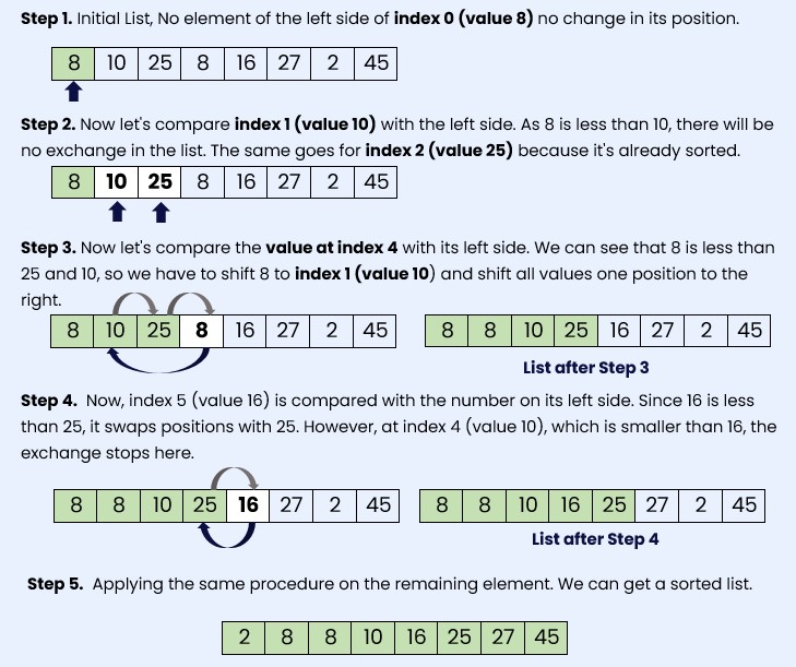
Question 2(a). Write an algorithm for insertion sort. Write step by step working of this algorithm for sorting the following list of data:
8,10,25,8,16,27,2,45 (10 marks)

Answer:

Inputs: A list of elements to be sorted.

Output: The list sorted in non-decreasing order.

1. Start with the second element (index 1) of the list.
2. Compare the current element with the elements to its left.
3. Move the current element to its correct position in the sorted portion of the list by shifting larger elements to the right.
4. Repeat steps 2-3 for each element in the list, starting from the second element and moving towards the end.
5. Once all elements have been processed, the list will be sorted.

Step-by-step working of Insertion Sort for the list: 8, 10, 25, 8, 16, 27, 2, 45

2. (a) Write an algorithm for insertion sort. Write step by step working of this algorithm for sorting the following list of data:

8, 10, 25, 8, 16, 27, 2, 45

[10 marks]

Answer :

3. (a) Write an algorithm for adding two polynomials. [10 marks]

Answer:

To add two polynomials, we need to sum the coefficients of the terms with the same degree. Here's a step-by-step algorithm:

Algorithm: Adding Two Polynomials

1. Input:
→ Two polynomials $P(x)$ and $Q(x)$ represented as arrays of coefficients.
→ Let $P(x) = a_n x^n + a_{n-1} x^{n-1} + \ldots + a_1 x + a_0$
→ Let $Q(x) = b_m x^m + b_{m-1} x^{m-1} + \ldots + b_1 x + b_0$
→ The arrays $A$ and $B$ where:
→ $A = [a_n, a_{n-1}, \ldots, a_0]$
→ $B = [b_m, b_{m-1}, \ldots, b_0]$

2. Initialize:
→ Determine the maximum degree $k$ of the resulting polynomial $R(x)$:
→ $k = \max(n, m)$
→ Create an array $R$ of size $k + 1$ initialized to zero:
→ $R = [0, 0, \ldots, 0]$

3. Process Coefficients:
→ For $i$ from 0 to $k$:
→ If $i \leq n$ (i.e., within the range of polynomial $P$):
→ Add the coefficient of $P(x)$ to $R[i]$:
→ $R[i] = R[i] + A[n-i]$
→ If $i \leq m$ (i.e., within the range of polynomial $Q$):
→ Add the coefficient of $Q(x)$ to $R[i]$:
→ $R[i] = R[i] + B[m-i]$

4. Output:
→ The resulting polynomial $R(x)$ represented by the array $R$:
→ $R = [r_k, r_{k-1}, \ldots, r_0]$

Example:

Suppose $P(x) = 2x^2 + 3x + 1$ and $Q(x) = x^3 + 4x + 5$:
→ $P(x)$ is represented by $A = [2, 3, 1]$
→ $Q(x)$ is represented by $B = [1, 0, 4, 5]$

Step-by-Step Execution:

→ Determine $k = \max(2, 3) = 3$
→ Initialize $R = [0, 0, 0, 0]$
→ Process coefficients:
→ $R[0] = 0 + 1 = 1$ (from $Q(x)$)
→ $R[1] = 0 + 3 + 4 = 7$ (sum of coefficients of $P(x)$ and $Q(x)$)
→ $R[2] = 0 + 2 + 0 = 2$ (from $P(x)$)
→ $R[3] = 0 + 1 = 1$ (from $Q(x)$)

Resulting Polynomial:
→ $R(x) = x^3 + 2x^2 + 7x + 6$
→ The array $R$ representing $R(x)$ is $[1, 2, 7, 6]$

Therefore, the algorithm correctly computes the sum of two polynomials.

Code Example:

        def add_polynomials(A, B):
            n = len(A)
            m = len(B)
            k = max(n, m)
            R = [0] * (k + 1)
            
            for i in range(k + 1):
                if i < n:
                    R[i] += A[n-i-1]
                if i < m:
                    R[i] += B[m-i-1]
            
            return R
        

3. (b) Explain indexed sequential file organization with the help of an example. [10 marks]

Answer:

Indexed sequential file organization combines the benefits of sequential and direct access file structures. It maintains records sequentially on the disk while using an index to provide fast access to specific records.

Key Features:

1. Sequential Storage:
→ Records are stored in sequential order based on a primary key field, such as an account number or ID.

2. Index Structure:
→ An index is maintained separately, containing pointers to the disk blocks or file offsets where each record starts.
→ Typically, this index is organized as a B-tree or B+ tree for efficient search and retrieval.

3. Access Mechanism:
→ Sequential access is primarily used for scanning through records in order.
→ Direct access via the index allows quick retrieval of specific records without scanning the entire file.

Example:

Consider a customer database stored using indexed sequential file organization:

Database Schema:
→ Each record contains fields like CustomerID, Name, Address, and Phone.

File Structure:
→ Records are sorted by CustomerID.

Index:
→ An index structure maintains pointers to the disk blocks or file offsets where each CustomerID's record begins.

Access Scenario:
→ To retrieve details of CustomerID 1234:
→ Use the index to quickly locate the disk block or offset containing the record for CustomerID 1234.

Indexed sequential file organization optimizes both sequential data access and direct record retrieval, making it suitable for applications requiring efficient search operations alongside sequential data processing.

4. (a) Traverse the following binary tree in pre-order and post-order: [10 marks]

Answer :

Pre-order Traversal

In pre-order traversal, we visit nodes in the order: Root, Left, Right.
$1. \ Visit \ A$
$2. \ Visit \ B$
$3. \ Visit \ C$
$4. \ Visit \ D$
$5. \ Visit \ E$
$6. \ Visit \ F$
$7. \ Visit \ G$
$8. \ Visit \ H$

So, the pre-order traversal of the tree is: A, B, C, D, E, F, G, H.

Post-order Traversal

In post-order traversal, we visit nodes in the order: Left, Right, Root.
$1. \ Visit \ C$
$2. \ Visit \ E$
$3. \ Visit \ D$
$4. \ Visit \ B$
$5. \ Visit \ G$
$6. \ Visit \ H$
$7. \ Visit \ F$
$8. \ Visit \ A$

So, the post-order traversal of the tree is: C, E, D, B, G, H, F, A.

4. (b) What is a Red-Black tree? Explain the properties of Red-Black tree. Explain how a node is inserted in a Red-Black tree. [10 marks]

Answer:

A Red-Black tree is a balanced binary search tree with additional properties that ensure the tree remains balanced after insertions and deletions.

Properties of Red-Black Tree:

1. Coloring:
→ Each node is either red or black.

2. Root Property:
→ The root is black.

3. Red Property:
→ Red nodes cannot have red children (no consecutive red nodes).

4. Black Depth Property:
→ Every path from a node to its descendant NULL nodes (leaves) must have the same number of black nodes (black height).

Insertion in Red-Black Tree:

1. Insertion Process:
→ Insert the new node as in a standard binary search tree based on its key value.

2. Coloring Rules:
→ Color the new node red initially.
→ Ensure the Red-Black properties are maintained by potentially rotating and recoloring nodes.

3. Maintain Balance:
→ After insertion, if necessary, perform rotations and recoloring to balance the tree and maintain the Red-Black properties.

Example:

Consider inserting a node with key value 15 into a Red-Black tree:

Initial Tree:
→ Assume a valid Red-Black tree structure.

Insert Node:
→ Insert node with key 15 following standard BST insertion.
→ Color the new node red.

Check Red-Black Properties:
→ Ensure no consecutive red nodes exist.
→ Check black depth consistency from the newly inserted node to all leaves.

Adjust Tree if Necessary:
→ Perform rotations and recoloring as needed to restore Red-Black tree properties.

The insertion process in a Red-Black tree guarantees balanced operations with logarithmic time complexity for insertions, deletions, and lookups, making it efficient for dynamic data structures.

Question 5(a). Write and explain Algorithm for binary search. Also, explain applications of binary tree. (10 Marks)

Answer:

Input:

• A sorted array arr of size n.
• The target element target to search for.

Output:The index of the target element if found, otherwise -1.

1. Set left to 0 and right to n - 1.
2. Repeat until left is less than or equal to right:
3. Calculate the middle index: mid = (left + right) / 2.

→ If arr[mid] equals target, return mid.
→ If arr[mid] is greater than target, set right to mid - 1.
→ If arr[mid] is less than target, set left to mid + 1.

4. If the target element is not found, return -1.

Explanation:Binary search is a divide and conquer algorithm used to find the position of a target element within a sorted array. The algorithm compares the target element with the middle element of the array. If they are equal, the search is successful. If the target element is less than the middle element, the search is performed in the left half of the array. If it is greater, the search is performed in the right half. This process continues recursively until the target element is found or the search space is empty.

Applications of Binary Search:

Question 5(b). What is Breadth First Search (BFS) ? Explain the difference between BFS and Depth First Search (DFS). (10 Marks)

Answer:

Breadth First Search (BFS) is a graph traversal algorithm that explores a graph level by level. Starting from a given source vertex, BFS systematically explores all the vertices reachable from the source vertex by visiting neighbors of the current vertex before moving on to the neighbors' neighbors. BFS is implemented using a queue data structure to keep track of the vertices that need to be visited next. BFS is commonly used to find the shortest path between two vertices in an unweighted graph.

Difference between BFS and Depth First Search (DFS):

Traversal Order: BFS explores the vertices level by level, visiting all the neighbors of a vertex before moving to the next level. DFS explores the vertices depth by depth, visiting as far as possible along each branch before backtracking.

Data Structure: BFS uses a queue to keep track of the vertices that need to be visited next, ensuring that vertices are visited in the order they were discovered. DFS uses a stack or recursion to keep track of the vertices that need to be visited next, resulting in a depth-first exploration of the graph.

Memory Usage: BFS typically requires more memory compared to DFS because it needs to store all the vertices at the current level in the queue. DFS can be implemented using less memory, especially when implemented recursively, as it only needs to store the vertices along the current path.

Completeness: BFS is guaranteed to find the shortest path between two vertices in an unweighted graph if one exists. DFS does not guarantee finding the shortest path, but it can be useful for certain tasks such as topological sorting and finding connected components.

Applications: BFS is commonly used for tasks such as finding the shortest path in unweighted graphs, network broadcasting, and finding connected components. DFS is commonly used for tasks such as topological sorting, cycle detection, and maze solving.

In summary, BFS and DFS are both graph traversal algorithms with different exploration strategies. BFS explores the graph level by level using a queue, while DFS explores the graph depth by depth using a stack or recursion. The choice between BFS and DFS depends on the specific requirements of the problem and the characteristics of the graph.